Probability Distribution of Tunnel Cost Overruns

In 2004 Bent Flyvbjerg published a guidance document titled Procedures for Dealing with Optimism Bias in Transport Planning. He’s got a lot of good analysis and plots, but one in particular brought a question to mind:

If someone tells me a project will cost 1 billion dollars, what cost should I expect by the time the project is over?

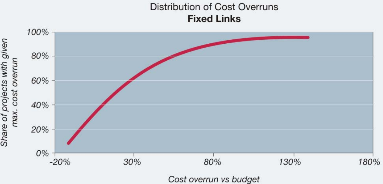
The plot that brought this to mind is a cumulative distribution function of cost overruns for tunnel and bridge projects:

To answer my original question, I decided to determine the expected value for the cost factor, and some confidences associated with this CDF. This way I can calculate the upper and lower bounds of the “most probable” cost. It doesn’t offer total certainty, but is much better than the one-number price that I know will be wrong.

If you don’t want to read on, the answer:

I should expect a $1 billion project to cost $1.3 billion, and should not be terribly surprised if the cost exceeds $2 billion.

Extract and re-plot the data

I first wanted to extra data from the plot into something more useful, like a .csv. So used this free plot digitizer to create scatter data representing the plot. Then recreated the plot to make sure my scatter data was correct:

Some key things that stick out:

74% of projects go over budget
23% of projects cost at least 1.5 times their original budget
6% of projects cost at least 2 times than the original budget
The median project goes 19% over budget

So, if you see a project budget in a newspaper for a new road or bridge, there is a 74% chance that it will end up costing more, most likely about 20% more.

Determine the distribution function

Most of the distribution functions to pick from don’t work very well when$x<0$, so I updated the x-axis values to be the “Cost Factor”: the number you multiply the quoted by to get the final price. I also wanted to fill out the plot so that there were values for 0% and 100%. Here is the updated plot (notice the single scatter points at the extreme left and right of the plot):

Now, I can use the python library scipy to determine the distribution. I’ll follow these steps:

• Make some dummy data from the CDF.
• Plot various distributions over the CDF.
• Visually determine which distribution fits best (I probably should do some additional goodness-of-fit testing…)

Make some dummy data:

def inverse_cdf(u: float) -> float:
    "Perform a linear interpolation using `CDF` as the `x` and `CostFactor` as the `y`"
    return np.interp(u, df["CDF"], df["CostFactor"])

# Generate N random numbers between 0 and 1 (0% and 100%)
N = 10000 
uniform_random_numbers = np.random.uniform(0, 1, N)

# Apply `inverse_cdf()` to the random numbers to create data that will follow
# the CDF above
random_variables = [inverse_cdf(u) for u in uniform_random_numbers]

Here’s what the data looks like in a histogram:

Now I use scipy to plot various distribtuions to see how they fit:

# Define the range of x-values to use in the distributions
cdf_x = np.linspace(df["CostFactor"].min(), df["CostFactor"].max())

# Fit the data to 5 different distributions using the scipy library
# For example: `stats.gamma.fit()` fits the data and provides the associated
# parameters for the `gamma` distribution function. `stats.gamma.cdf` uses the
# parameters and the x-range to calculate an array that represents the CDF
cdf_gamma = stats.gamma.cdf(cdf_x, *stats.gamma.fit(random_variables))
cdf_weibull_min = stats.weibull_min.cdf(cdf_x, *stats.weibull_min.fit(random_variables))
cdf_weibull_max = stats.weibull_max.cdf(cdf_x, *stats.weibull_max.fit(random_variables))
cdf_exponweib = stats.exponweib.cdf(cdf_x, *stats.exponweib.fit(random_variables))

# Add the CDFs to the original scatter plot
for name, trace in {
    "gamma": cdf_gamma,
    "weibull_min": cdf_weibull_min,
    "weibull_max": cdf_weibull_max,
    "exponweib": cdf_exponweib,
}.items():
    fig_cdf.add_trace(go.Scatter(x=cdf_x, y=trace, name=name, mode="lines"))

fig_cdf.update(layout=dict(legend=dict(yanchor="top", y=0.99, xanchor="left", x=0.01)))

fig_cdf.show()

From a visual check, all but the weibull maximum extreme value distribution seem to be very close. For the remainder of this exercise I will assume the gamma distribution, mostly because it looks like a reasonable fit.

Determine the expected value and confidence interval

Thankfully scipy makes this pretty easy by way of the .expect() and .interval() methods for their rv_continuous class:

# Calculate the distribution expected value and 95% confidence interval
expected_value = stats.gamma(*stats.gamma.fit(random_variables)).expect()

# Define the range of confidence intervals to use
ci_range = np.linspace(0.5, 0.99)

# Calculate the confidence intervals using the `gamma.fit` method and the same
# `random_varialbes` used previously
ci_vals = [
    (i, *stats.gamma(*stats.gamma.fit(random_variables)).interval(i)) for i in ci_range
]

# Make a `dataframe` and add the expected value column for plotting
df = pd.DataFrame(ci_vals, columns=["CI", "Lower", "Upper"])
df["Expected Value"] = expected_value

# Plot the figure
fig = (
    px.line(df, x="CI", y=["Lower", "Upper", "Expected Value"])
    .update(
        layout=dict(
            title="<b>Confidence interval and cost factor</b><br><i>Fixed Links (bridges and tunnel)</i>",
            height=500,
            width=800,
            margin=dict(t=60, b=20, l=20, r=20),
            legend=dict(title="Bound", yanchor="top", y=0.99, xanchor="left", x=0.01),
            xaxis=dict(title="Confidence Interval"),
            yaxis=dict(title="Cost Factor"),
        )
    )
    .add_annotation(
        text=f"<b>Expected Value = {round(expected_value, 2)}</b>",
        showarrow=False,
        xref="paper",
        x=0.75,
        yref="paper",
        y=0.25,
    )
)

Conclusion

Back to the original question:

If someone tells me a project will cost 1 billion dollars, what cost should I expect by the time the project is over?

To answer this, I:

• Extracted data from a .png of a CDF depicting the cost overruns for bridge and tunnel projects.
• Determined a reasonably representative distribution function that can be used to mathematically describe the published CDF.
• Use the distribution function to determine the expected value and confidence intervals.
• Plotted the confidence intervals (upper and lower bounds) in respect to the confidence value (50% to 99%).

The answer:

I should expect a $1 billion project to cost $1.3 billion, and should not be terribly surprised if the cost exceeds $2 billion.